{lvmisc} has a set of tools to work with statistical model objects. Generally, the functions behind these tools are S3 generic and the methods currently implemented are for the classes lm from the {stats} package and lmerMod from the {lme4} package. If you would like to have methods implemented to other model classes, please file an issue at https://github.com/verasls/lvmisc/issues.
The functions to work with models can be divided into three categories:
- Model diagnostics
- Model cross-validation
- Model accuracy
Before starting, let’s load the required packages:
Model diagnostics
{lvmisc} has a plotting function for some common model diagnostic plots. To explore it, let’s first create some example models:
The main function to generate the diagnostic plots is plot_model() and its only argument is the model object:
plot_model(m1)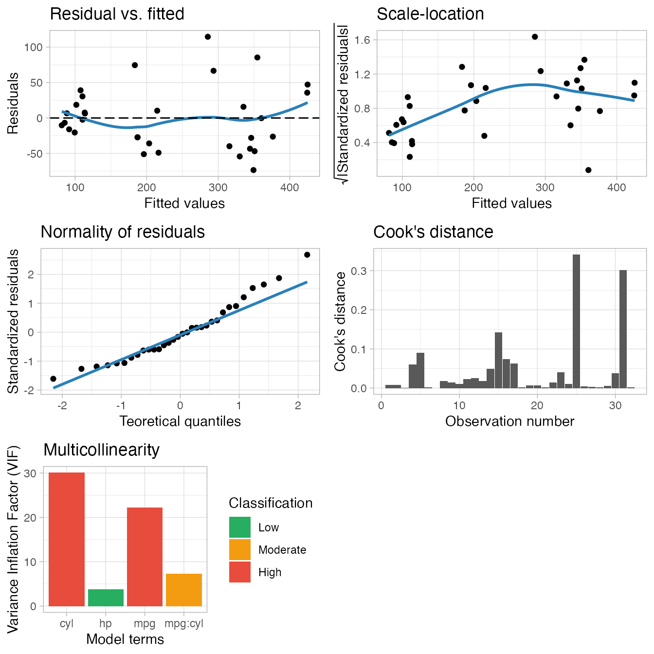
plot_model(m2)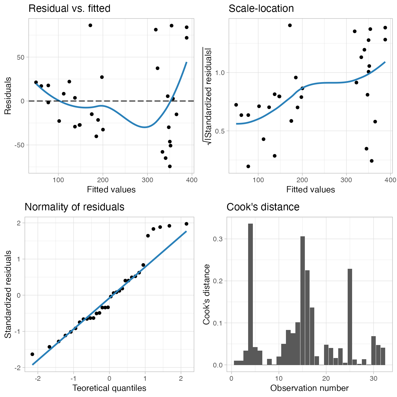
By default it prints a grid of five (or four) diagnostic plots. Each individual plot can also be generated by using another function. The default plots shown are, respectively:
- A scatterplot of the residual vs. fitted values, with a smoothing line, which is useful to show if the residuals have a non-linear pattern. In this plot, the points should be randomly distributed around the smoothing line, and the smoothing line should be approximately horizontal and around the 0 line.
plot_model_residual_fitted()generates this plot. - A scatterplot of the square root of the absolute value of the model residuals vs. the fitted values, with a smoothing line. In this plot, again you should look for a horizontal smoothing line with the points randomly distributed around it, if it’s the case, you can assume the homogeneity of variance of the residuals.
plot_model_scale_location()generates this plot. - A Q-Q plot of the standardized residuals, showing if the residuals are normally distributed. Normality is assumed if the residuals are well aligned with the straight blue line.
plot_model_qq()generates this plot. - A bar plot with the Cook’s distance per observation. This is a useful plot to check for influential observations. A given observation is often considered to be influential in the model if its Cook’s distance is higher than 1.
plot_model_cooks_distance()generates this plot. - A bar plot with the variance inflation factor (VIF) per model term, which only shows if the model has 2 terms or more (you can see that in our example this plot is not built for
m2). The VIF can be used to check the model for multicollinearity: the bar is green for a low multicollinearity, orange for moderate and red for high.plot_model_multicollinearity()generates this plot.
Model cross-validation
The cross-validation of a model is a way to assess how the results of a statistical model will generalize to an independent data set, but without the burden of collecting more data. At the moment, the only cross-validation method available in the {lvmisc} package is the leave-one-out. Also, the only model classes supported are lm and lmerMod, but more cross-validation methods and classes will be implemented in the future.
The leave-one-out cross validation method works by each subject’s data into a testing dataset (one participant at a time) with the remaining data being the training dataset. New models with exactly the same specifications as the original model are developed using the training dataset and then used to predict the outcome in the testing dataset. This process is repeated once for every subject in the original data.
We will now build a linear model to demonstrate the cross-validation with the loo_cv() function.
# Put the rownames into a column to treat eat row as a "subject" (car) in
# the leave-one-out cross-validation
mtcars$car <- row.names(mtcars)
m <- lm(disp ~ mpg, mtcars)
loo_cv(model = m, data = mtcars, id = car, keep = "used")
#> # A tibble: 32 x 3
#> car .actual .predicted
#> <chr> <dbl> <dbl>
#> 1 Dodge Challenger 318 310.
#> 2 Ferrari Dino 145 241.
#> 3 Toyota Corolla 71.1 -30.3
#> 4 AMC Javelin 304 317.
#> 5 Duster 360 360 330.
#> 6 Merc 450SLC 276. 318.
#> 7 Camaro Z28 350 349.
#> 8 Merc 450SE 276. 296.
#> 9 Pontiac Firebird 400 241.
#> 10 Merc 280C 168. 274.
#> # … with 22 more rowsTo use the loo_cv() function you need to specify the model you will cross-validate, the original dataset used to build it and the name of the column which identifies the subjects. You will also notice the use of the keep argument: it controls the columns to be shown in the output object (more details in the loo_cv() documentation).
The output of the cross-validation function is an object of class lvmisc_cv. It is simply a tibble with at least two columns: one containing the dependent variable actual values (.actual) as in the original dataset, and the other with the values predicted by the cross-validation procedure (.predicted). These two columns contain the data necessary to evaluate the model performance, as we will see in the next section.
Model accuracy
{lvmisc} also has an easy method to compute the most common model accuracy indices (accuracy() function) and to compare the accuracy indices of different models (compare_accuracy() function). Similarly to the other {lvmisc} functions described in this vignette, it has methods for the lm and lmerMod classes and also for the lvmisc_cv class.
To explore the accuracy() function, let’s use the same models built in the first example of this vignette.
m1 <- lm(disp ~ mpg + hp + cyl + mpg:cyl, mtcars)
m2 <- lmer(disp ~ mpg + (1 | cyl), mtcars)
# Let's also cross-validate both models
cv_m1 <- loo_cv(m1, mtcars, "car", keep = "used")
cv_m2 <- loo_cv(m2, mtcars, "car", keep = "used")And then use the accuracy() function in each of the models to compute their accuracy indices.
accuracy(m1)
#>      AIC    BIC   R2 R2_adj  MAE   MAPE  RMSE
#> 1 344.64 353.43 0.87   0.85 34.9 15.73% 43.75
accuracy(m2)
#>      AIC    BIC R2_marg R2_cond   MAE   MAPE  RMSE
#> 1 340.76 346.62    0.19    0.81 35.75 16.43% 44.31
accuracy(cv_m1)
#>      AIC    BIC   R2 R2_adj   MAE   MAPE  RMSE
#> 1 344.64 353.43 0.87   0.85 41.82 18.59% 52.58
accuracy(cv_m2)
#>      AIC    BIC R2_marg R2_cond   MAE   MAPE  RMSE
#> 1 340.76 346.62    0.19    0.81 40.77 19.06% 50.28
As can be seen, the accuracy() function returns the following accuracy indices: Akaike information criterion (AIC), Bayesian information criterion (BIC), R2 values appropriate to the model assessed, mean absolute error (MAE), mean absolute percent error (MAPE) and root mean square error (RMSE).
Examining the accuracy results above we can see that the AIC, BIC and R2 values do not change between the cross-validated model and the original model (e.g. m1 vs. cv_m1 and m2 vs. cv_m2). This happens because the AIC, BIC and R2 for an object of class lvmisc_cv are computed based on the original model. It can also be observed that the MAE, MAPE and RMSE values are worse for the cross-validated model, which is expected, as it is used to test an “out-of-sample” performance.
Furthermore, we can also compare the accuracy indices of different models using the compare_accuracy() function.
compare_accuracy(m1, cv_m1, m2, cv_m2)
#> Warning: Not all models are of the same class.
#> Warning: Some models were refit using maximum likelihood.
#>   Model                   Class   R2 R2_adj R2_marg R2_cond    AIC    BIC   MAE
#> 1    m1                      lm 0.87   0.85      NA      NA 344.64 353.43 34.90
#> 2 cv_m1      lvmisc_cv_model/lm 0.87   0.85      NA      NA 344.64 353.43 41.82
#> 3    m2                 lmerMod   NA     NA    0.28    0.76 353.90 359.77 36.03
#> 4 cv_m2 lvmisc_cv_model/lmerMod   NA     NA    0.19    0.81 340.76 346.62 40.77
#>     MAPE  RMSE
#> 1 15.73% 43.75
#> 2 18.59% 52.58
#> 3 16.77% 44.47
#> 4 19.06% 50.28
Some of the benefits of using this function instead of manually comparing models with several accuracy() calls are that compare_accuracy() output shows the models info (object name and class) and it throws warnings to aid the comparison.